What is the practical difference between linear, decaying, and halving emissions?
Emission schedules are incentive contracts. They decide who gets paid for arriving early, who absorbs dilution, and how abruptly the network tests whether participation is still worth it. In staking systems, emissions are part of the public reward policy, and reward levels interact with the amount of capital locked versus liquid capital left in the market, as discussed in staking research.
| Model | Shape | What it rewards | Main risk | Concrete example |
|---|---|---|---|---|
| Linear | Equal absolute change per period | Predictable participation and budgeting | Can keep overpaying even after growth slows | Sia launched with a 300,000 SC block reward, reduced it by 1 SC per block, and stopped the decline at 30,000 SC from block 270,000 onward in its block reward schedule. |
| Decaying | Percentage reduction over time | Early bootstrapping with gradual tapering | Still open-loop if the network’s real security needs change | Solana’s inflation schedule starts at 8% annual inflation, declines by 15% year over year, and targets a 1.5% long-run rate. |
| Halving | 50% cut at fixed intervals | Scarcity discipline and operator efficiency | Large step-changes in operator revenue | Bitcoin’s block subsidy is cut in half every 210,000 blocks. |
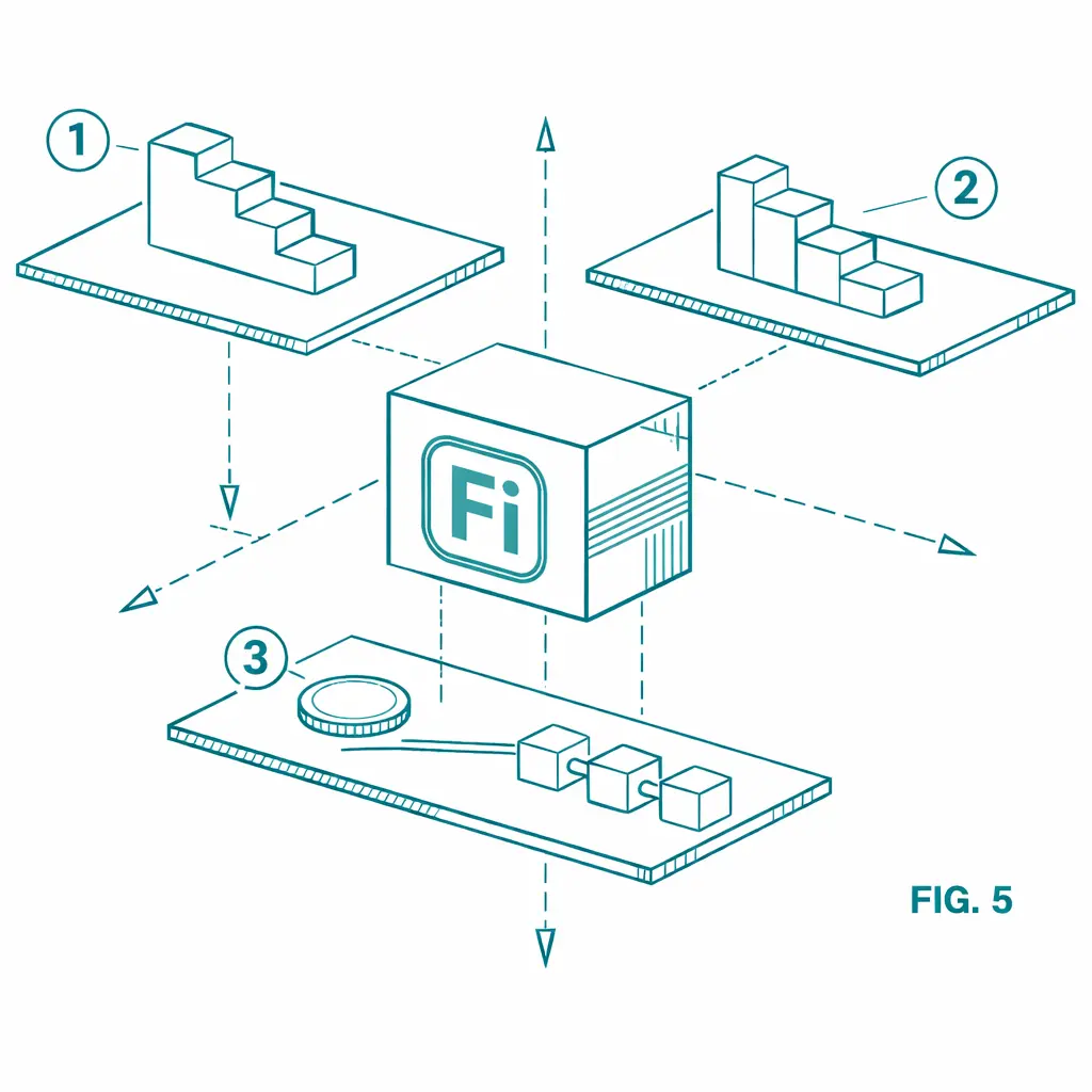
Halving is best understood as stepwise decay. Decaying schedules reduce issuance more smoothly. Linear schedules move by equal absolute amounts, which can mean a constant release or a straight-line decline. The economic difference is not cosmetic. A smooth curve changes behavior gradually. A halving forces a sudden repricing of security, liquidity, and expected sell pressure.
Which behaviors does each schedule reward?
Linear emissions reward predictability. Operators, farmers, or validators can model revenue easily because the schedule moves in fixed absolute increments. That helps when the system wants stable participation or a clearly budgeted subsidy runway. The problem is incentive drift. If demand, fees, or network usage do not catch up, the chain can keep paying the same style of subsidy long after that subsidy stopped buying useful behavior. Sia’s design shows the virtue and the trade-off clearly: the reward declines mechanically, then persists forever at a fixed floor.
Decaying emissions reward early participation without promising permanent generosity. This is often the cleanest fit for networks that need to bootstrap validators, liquidity, or users early and then taper support as the system matures. Solana’s public inflation design is explicit about this logic: inflation funds delegated stake accounts and validators, and expected staking yield depends heavily on the fraction of SOL staked. That is better aligned than a blind fixed payout because the schedule acknowledges that early security bootstrapping and mature-state security are not the same problem. That is why staking rewards and risks have to be modeled together.
Halving rewards conviction and cost discipline. Everyone knows the shock date is coming. Efficient operators survive. Marginal operators get squeezed. Holders get a stronger scarcity story. That structure can be powerful if the network wants monetary hardness to be legible and non-negotiable. It is weaker when the system still depends on subsidy to keep supply-side participants online. Bitcoin’s schedule is credible precisely because the rule is simple and hard to reinterpret. The trade-off is that revenue compression happens in cliffs, not slopes.
How do these schedules change dilution and sell pressure?
Emissions dilute passive holders unless they are offset by real demand, real fee income, or real security value. In PoS systems, that dilution is not abstract. New supply is routed to stakers and validators, while unstaked holders absorb the inflation. Solana states this directly: 100% of inflationary issuance is proposed to go to delegated stake accounts and validators, and staking yield depends primarily on the fraction of SOL staked. More generally, real yield versus emissions sits inside the stake-versus-liquidity trade-off, because new token issuance expands supply and changes relative positioning.
Linear schedules usually create the most persistent sell pressure if the absolute token flow remains large relative to organic demand. Decaying schedules reduce that pressure gradually. Halving models reduce issuance fastest in discrete steps, but they can create sharp post-event revenue stress for miners or validators. That is the core trade-off: smoother dilution versus sharper operating shocks. If the network wants a permanent security budget instead of a race toward fee-only security, Monero shows the opposite endpoint. Its tail emission keeps block rewards at 0.6 XMR or less per block rather than letting rewards fall to zero.
The incentive-alignment test is simple. If emissions are high enough to attract participation but too vague to measure what participation actually contributes, the schedule starts rewarding extraction. A validator, miner, or yield farmer who is paid regardless of marginal value will rationally harvest the subsidy and sell. Emission design fails when it pays for presence instead of performance.
Which schedule is strongest for network security?
No schedule is universally strongest. Security depends on what must be paid for, how observable that contribution is, and whether fee revenue can replace subsidy before operators exit. For PoW systems, the long-run question is especially hard. Princeton researchers showed that a regime dominated by transaction fees creates new attack incentives, including undercutting and more effective selfish-mining variants, and argued that permanent block rewards may be a reasonable price for stability. That does not invalidate Bitcoin’s design. It does show that “we will just live on fees later” is not a trivial assumption.
For PoS and service networks, decaying schedules usually age better than halving schedules because they reduce subsidy without forcing a single hard revenue cliff. That is one reason modern PoS systems often separate the question of how much inflation exists from how rewards respond to participation. Kusama’s inflation model is explicit: inflation is 10% annually, but the share routed to stakers versus treasury changes dynamically around an ideal staking rate, with the mechanism designed to incentivize more staking below target and less staking above target.
The important implication is that fixed schedules are open-loop. They do not know whether the network is undersecured, overpaying, or suffering from illiquidity. If your core problem is hitting a target participation ratio, a dynamic mechanism can be more aligned than any fixed linear, decaying, or halving path. Fixed curves are strongest when the network values credibility and simplicity more than adaptiveness.
When is each model the wrong choice?
Linear is the wrong choice when product-market fit is uncertain and the network cannot justify steady absolute issuance for long. In that case, predictability for insiders becomes a tax on everyone else.
Decaying is the wrong choice when the terminal rate is reached before fees, usage, or non-emission rewards can keep participants engaged. A graceful curve still fails if the destination is underfunded.
Halving is the wrong choice when the network cannot tolerate abrupt cuts to validator or miner revenue. If security depends on continuity more than on scarcity theater, halving is too blunt an instrument.
Any fixed schedule is the wrong choice when the real objective is maintaining a target stake ratio, validator set quality, or service capacity. That is a control problem, not a branding problem. Dynamic reward policies exist because static curves frequently overpay in one regime and underpay in another.
What decision rule should teams actually use?
Start with the behavior you need to buy, not with the chart you want to market. If the network needs a temporary bootstrap, choose a decaying curve. If it needs maximum monetary legibility and can survive periodic subsidy shocks, halving is coherent. If it needs budget certainty for a known operating runway, linear can work. If it needs to hold participation near a target, stop pretending this is a fixed-schedule problem and design a responsive mechanism instead. That choice still sits inside broader token supply decisions.
The cleanest token economy design process asks four questions in order: who receives new tokens, what measurable behavior they provide in return, how much sell pressure the market can absorb, and what happens when emissions stop feeling generous. That is where most bad tokenomics fail. The curve is visible, but the incentive mapping is weak.
From FinDaS Tokenomics’ standpoint, this is also where serious tokenomics consulting adds value. The hard part is rarely choosing between linear, decaying, and halving in the abstract. The hard part is proving that the reward path keeps rewarding useful behavior after the first wave of easy growth is over.